Numerical Scheme

Numerical method

Spatial discretisation

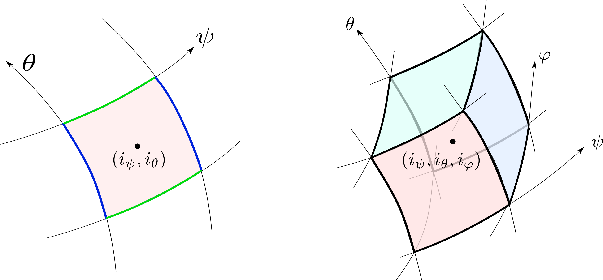
The numerical scheme of Soledge3X is based on 2D or 3D finite volumes. The grid is structured in the $(\psi,\theta,\varphi)$ coordinate system where $\psi$ is a radial coordinate, $\theta$ is a poloidal coordinate and $\varphi$ is a toroidal coordinate. Most of the time, $\psi$ is in fact associated with the magnetic flux and the grid is thus aligned with magnetic flux surfaces. The element cell of the grid is a quadrangle (in 2D) or a parallelepiped (in 3D) identified by its indices $(i_\psi, i_\theta, i_\varphi)$.

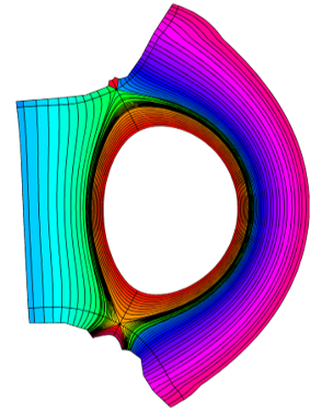
A domain decomposition is used to simulate X-point geometries. Each domain is called a “zone” and is given an index. A neighboring matrix specifies how zones communicate between each others in all directions. Examples of domain decomposition are plotted below for a single X-point, a double X-point and a snowflake configuration.

The following numerical methods are used to treat the different operators. To compute divergence of fluxes, the finite volume scheme requires fluxes at the boundary of the grid cells or half-points that can be indexed $(i_\psi \pm \frac{1}{2}, i_\theta, i_\varphi)$ for radial faces, $(i_\psi, i_\theta \pm \frac{1}{2}, i_\varphi)$ for poloidal faces, $(i_\psi, i_\theta, i_\varphi\pm \frac{1}{2})$ for toroidal faces:

• Advection: advection fluxes are computed by the Donat and Marquina scheme. This scheme requires plasma quantities estimated at the half-points (both sides). This is done by a 3rd order WENO interpolation of plasma fields.
• Parallel diffusion: parallel diffusion fluxes are computed with simple 2nd order finite difference for 2D simulations (in that case, the parallel gradient is in fact 1D in the $\theta$ direction). For 3D cases, the parallel gradient is computed within the flux surface across both the $\theta$ and $\varphi$ direction. The gradient is not aligned with the grid and the dedicated Günter scheme is used to reduce numerical diffusion.
• Perpendicular diffusion: perpendicular diffusion fluxes are computed with a simple 2nd order finite difference scheme. We use the preserving monoticity scheme for anisotropic diffusion proposed by Sharma and Hammett.

Once the fluxes are computed, the divergence is computed from its weak formulation integrated over the grid cell volume: $$\vec{\nabla}\cdot\vec{\phi} = \frac{1}{V_{\textrm{cell}}} \sum_{faces} \vec{\phi}\cdot \vec{S}{\textrm{face}}$$ where $V{\textrm{cell}}$ is the volume of the grid cell, $\vec{\phi}\cdot\vec{S}_\textrm{face}$ is the flux crossing a particular face multiplied by the face area.

Time advancement

Soledge3X relies on a mix explicitt-implicit scheme. The following terms are treated explicitely:

• Advection
• Perpendicular diffusion
• Source terms

The following terms are treated implicitely due to their fast dynamic that would reduce the time step too much:

• Parallel viscosity
• Parallel heat conduction
• Parallel current

In addition, since the electric potential equation takes the form $$\partial_t \vec{\nabla}\cdot(A \vec{\nabla}_\perp \phi) + \vec{\nabla} \cdot (\sigma_\parallel \nabla_\parallel \phi \vec{b}) = RHS$$

a part of time derivative of the perpendicular laplacian involves solving implicitely the perpendicular laplacian. Parallel viscosity, heat conduction and parallel current are 1D operators for 2D simulations and 2D operators for 3D simulations. Different sparse matrix solvers can be used to invert this set of 1D or 2D problems. Since the problems are not too big, direct solvers are usually applied such as LAPACK for the 1D problem or the PASTIX solver developped by INRIA for the 2D problems. For the electric potential equation, since one has to solve implicitely a parallel laplacian and a perpendicular laplacian, the problem couples all the points of the domain. For 2D simulations, the problem remains small and can be inverted with the direct solver PASTIX. For 3D simulations, the problem takes the form of a 3D sparse matrix to inverse and becomes very costly given that the strong anisotropy of diffusion makes the matrix poorly conditionned. The boundary conditions on the electric potential (Robin boundary condition almost degenerated to Neumann) add to the poor conditionning of the problem. Iterative solver are used to deal with this problem, the most efficient solver found so far being GMRES or BiCGStab coupled to an Algebraic Multi-Grid pre-conditionner. The following libraries have been tested and coupled to Soledge3X:

• AGMG developped at ULB
• PETSC used with the gamg pre-conditionner
• HYPRE used with BoomerAMG pre-conditionner

Parallelisation

The parallelisation of the computation relies on an hybrid MPI-OpenMP implementation. In addition to the “topological” domain decomposition mentionned above, each zone is redecomposed in small “chunks” which are small structured parts of the zone domain of size $N_{\psi,\textrm{chunk}}\times N_{\theta,\textrm{chunk}}\times N_{\varphi,\textrm{chunk}}$. The decomposition uses URB partitionning of the grid and all chunks do not necerally have exactly the same size but attempt to match a targeted number of points (e.g. 1024, 2048 points per chunk). Each process is given a set of chunks to deal with, sharing the work load and the memory needed to store the different fields among the different MPI processes. An example of decomposition of a 2D case into different chunks is represented in the figure below.

In addition to this MPI share of the domain, the set of chunks owned by each process is solved in parallel using OpenMP. If $N_\textrm{chunks}$ is the number of chunks a process has to deal with, the OpenMP parallelisation takes the form:

!$OMP DO
do ichunk = 1, Nchunks
   call solveChunk(ichunk)
end do
!$OMP END DO

Moreover, a great part of the computation can be parallelized over the different species in the plasma. Once again, OpenMP parallelisation is used to parallelize the species loop, most of the time gathering the chunk loop and the species loop together. Below is given a typical example of OpenMP loop in Soledge3X, the loop over species spannig from 0 (electrons) over all ion species including the different ionisation states:

!$OMP DO COLLAPSE(2)
do ichunk = 1, Nchunks
   do ispec = 0, Nspecies
      call solveChunk(ichunk,ispec)
   end do
end do
!$OMP END DO

Inside this loop, the solveChunk function will loop over the points contained within the chunk. No extra parallelisation layer applies at that level and one relies there on vectorisation performance. The solveChunk function will exhibit loops like:

subroutine solveChunk(ichunk,ispec)
	implicit none
	real(kind=dp), dimension(:,:,:), pointer :: A_ptr
	integer*4 :: ipsi, itheta, iphi
!...
! pointing to the chunk+spec data
	A_ptr => chunks(ichunk)%spec(ispec)%A
!...
! loop over points in the chunk
	do ipsi = 1, chunks(ichunk)%Npsi
	   do itheta = 1, chunks(ichunk)%Ntheta
	      do iphi = 1, chunks(ichunk)%Nphi
	      	 A_ptr(iphi,itheta,ipsi) = !...
	      end do
	   end do
   	end do
!...
end subroutine

Remark on the code performance

Despite the effort to improve the code speed-up, for “big” 3D cases, most of the computation time is spent within the libraries to solve the 3D electric potentital equation. Most of the effort to improve the code performance thus focus today on optimising the use of the available solvers as well as on improving the conditionning of the electric potential problem.

More details on the numerical scheme can be found in the code’s manual.